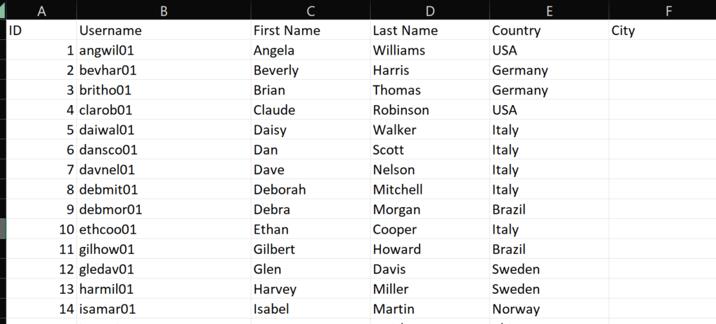
Creating sample data using Excel
From time to time I need to create a sample dataset. It might be for a demo to a customer, a talk at a conference, to test out a calculation or for a blog post for example. No matter what reason you might have, I want to show you how I usually create sample data using Excel!
A dimensional User table
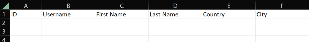
Start of with a blank Excel file and add some fields for a dimensional user table like this:
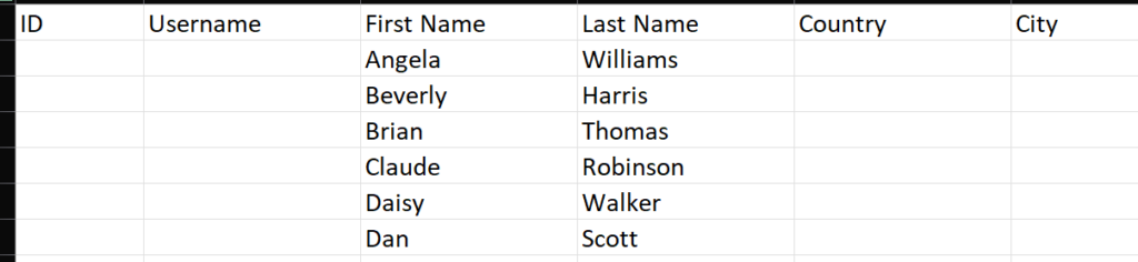
To fill in first and last names you can ask ChatGPT to generate a list of sample names or simply just google them.
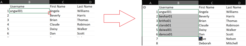
When you’ve added a couple of names to C and D, you list should look something like this and it’s time for ID and Username.
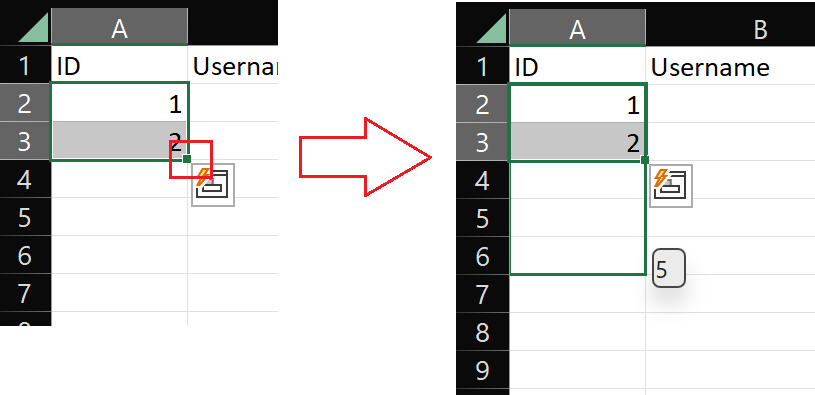
For ID we’ll make use of the fill function. Write 1 in the first row and 2 in the second, then select both, click and hold the left mouse key on the magical little square on the bottom right of the selection and just drag down to as many rows as you have names in your list. Voilà! One ID column with a unique number for each user.
A typical username is the first three letters of your first name and the first three of the last name followed by a number. The number could of course be calculated as well if my list had thousands of users and duplicates would be an issue. My list will be just a few users so I’ll just delete any duplicate values I might get from this. The formula for my user name is this and you can see the steps below that builds the formula.
=LOWER((LEFT(C2;3)&LEFT(D2;3)))&"01"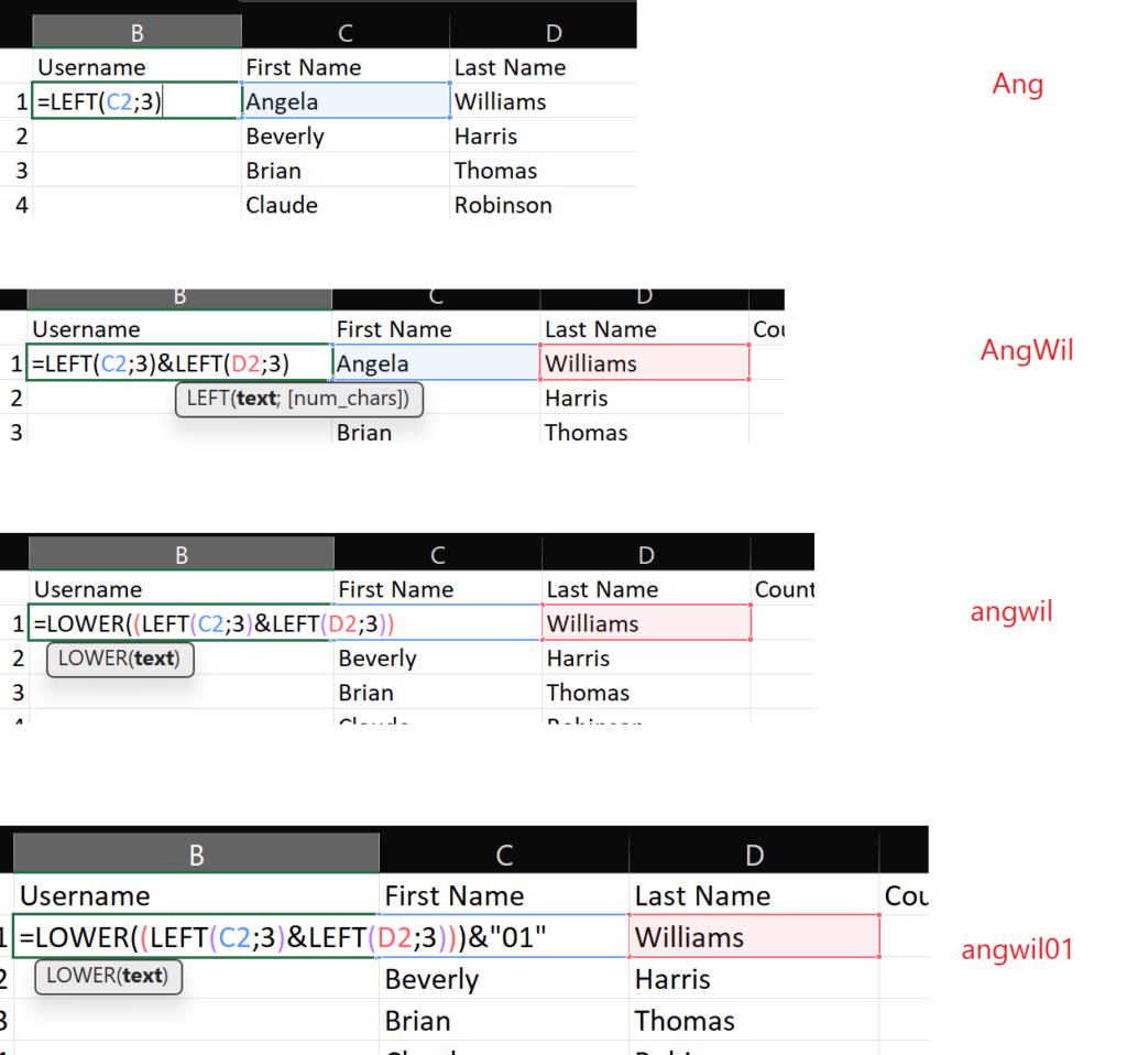
And again with the select, click and hold on the square and just drag down to copy the formula for each row. Another trick by the way, if you for example have a long list and feel like not wasting time to drag the selection all the way, just double click on the square and you will automatically fill all the way down as long as there is a value on the left side (in our case there is the ID number).
If you really want to make sure you have no duplicates in your list, a simple check is to conditionally format the column to highlight duplicate values. Select the whole of B, go to Home, Conditional formatting, highlight cells rules and select Duplicate values. Default they will show in red like this.
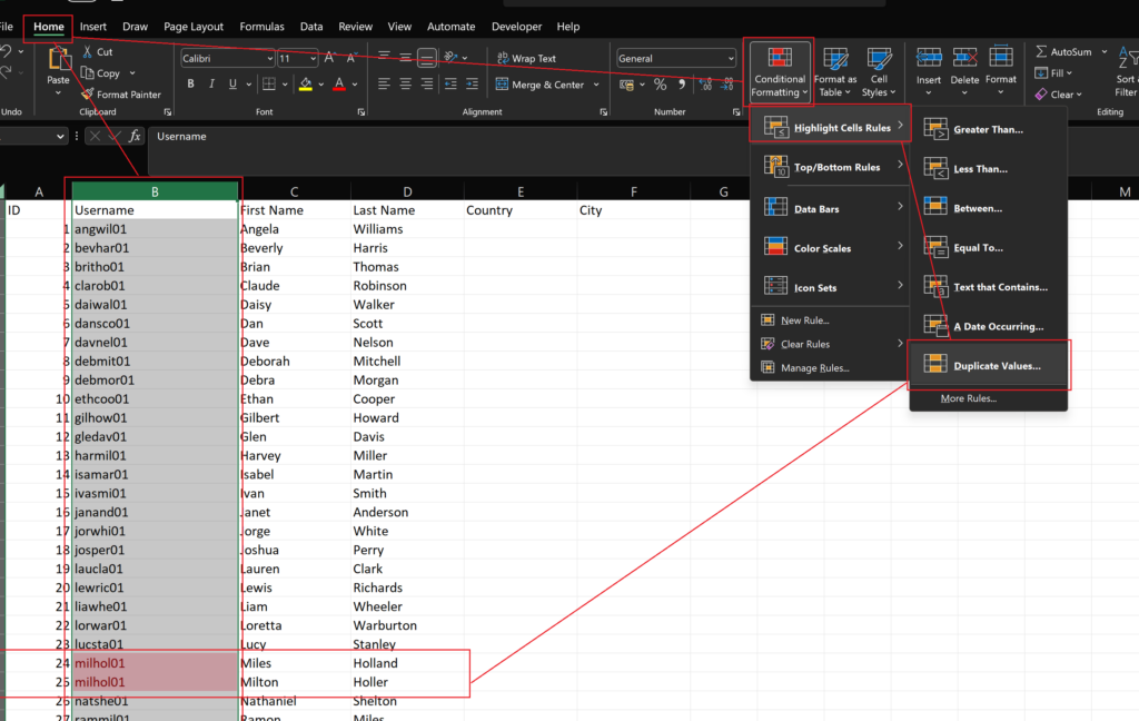
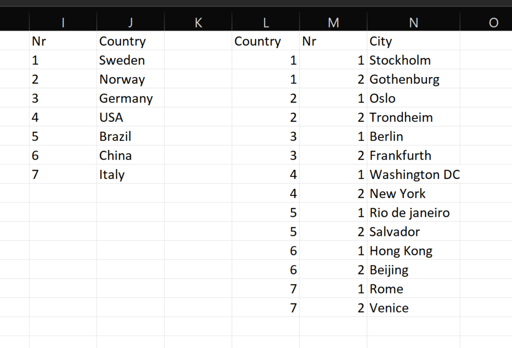
I changed the last name Holler to Smith and got rid of my duplicate. Moving on, we want to add country and city to the users on random.
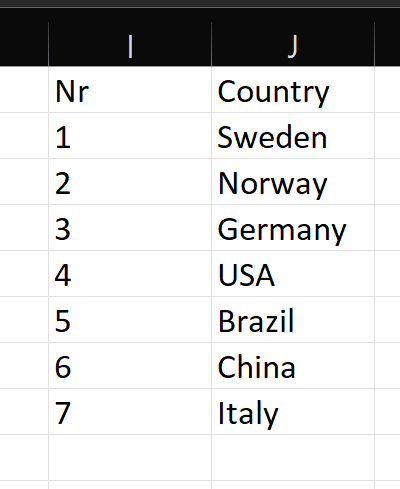
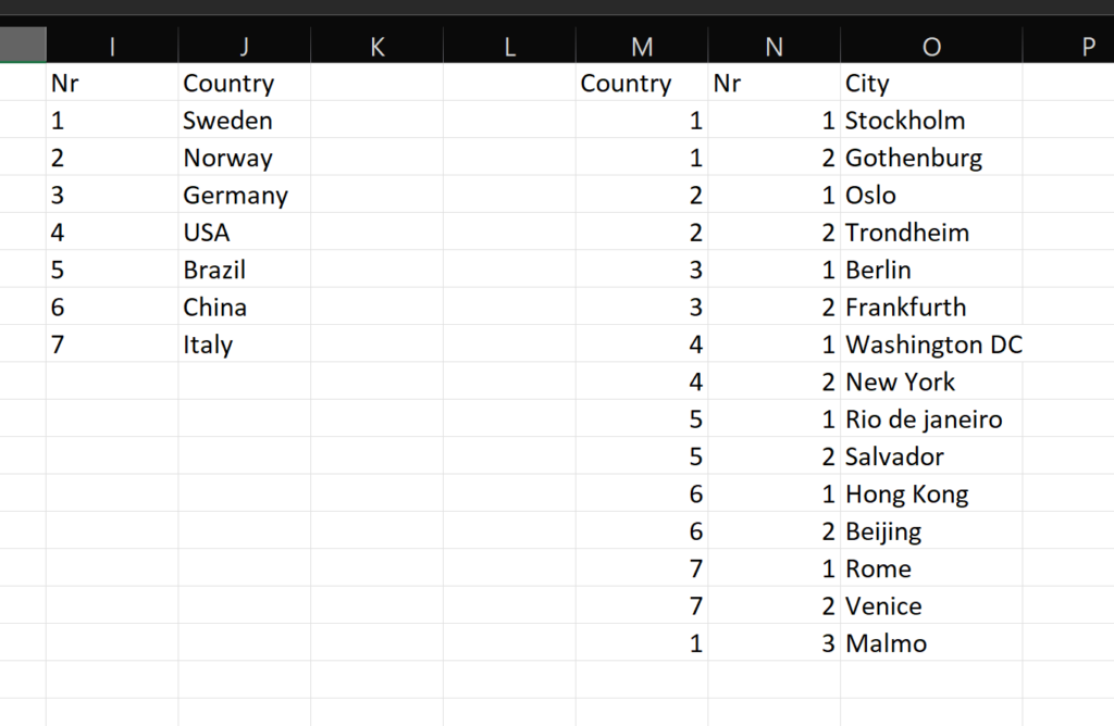
First, create a list of the countries we will be choosing from. Add an index to your country table like this.
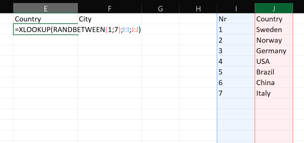
Now for some XLOOKUP magic! In the country column of the user table we want to add a country on random. The XLOOKUP needs to search for a value in a column or row and will return a value from the same row or column as the value that was found. We know that we have 7 countries in our list, so we can use RANDBETWEEN to randomly generate a number between 1 and 7 for each row in our user table!
The user list starts to look pretty good! But we want a city as well and here we don’t just want to select a random city. We want a random city within each country.
I’ve added this list where each country is represented on 2 records, each city has a unique Nr ID for each country. I only have 2 cities per country here so they’re just alternating between 1 and 2.
Hold on to your hats because it’s about to be slightly more advanced here. Promise that this is as deep as we’ll dive into Excel formulas for this blog post though!
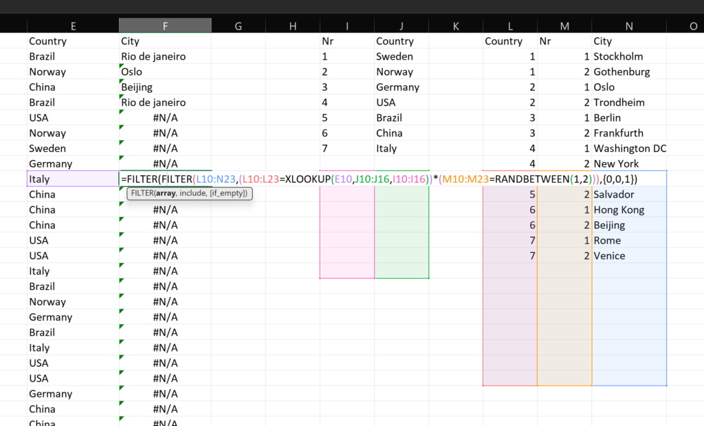
What we want to do is filter out the city rows for the country randomly selected for the user on each row and the randomly select one of the 2 cities.
Here’s the formula that will do it and a print screening proof. An explanation will follow 😉
=FILTER(FILTER(L$2:N$15,(L$2:L$15=XLOOKUP(E2,J$2:J$8,I$2:I$8))*(M$2:M$15=RANDBETWEEN(1,2))),{0,0,1})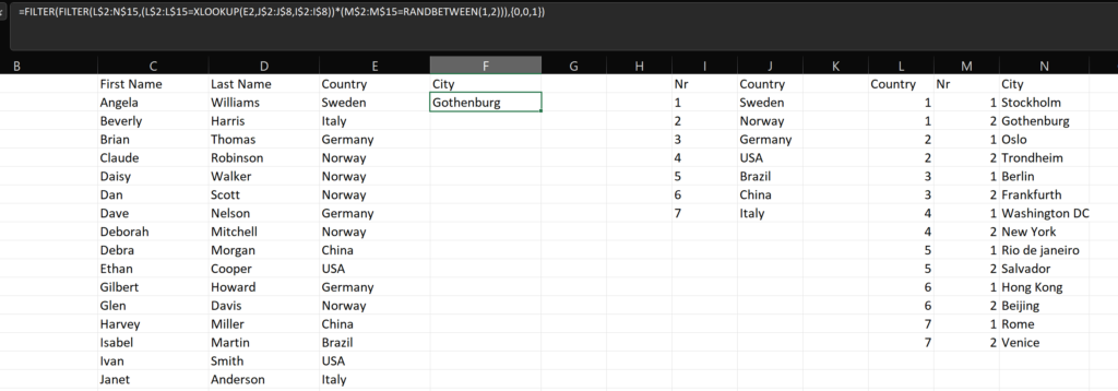
In Excel you cant line break in a formula, but if we were to write it out that way it might look something like this.
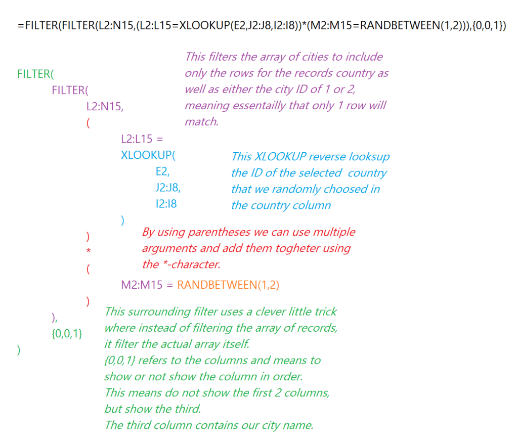
This will not work though, as each formula will reference a new array relative to the row number. Example here:
To solve it, you need to lock the formula reference using a dollar sign before the row numbers that we want to stick. We haven’t used this before since we’ve referenced the entire column in the previous examples.
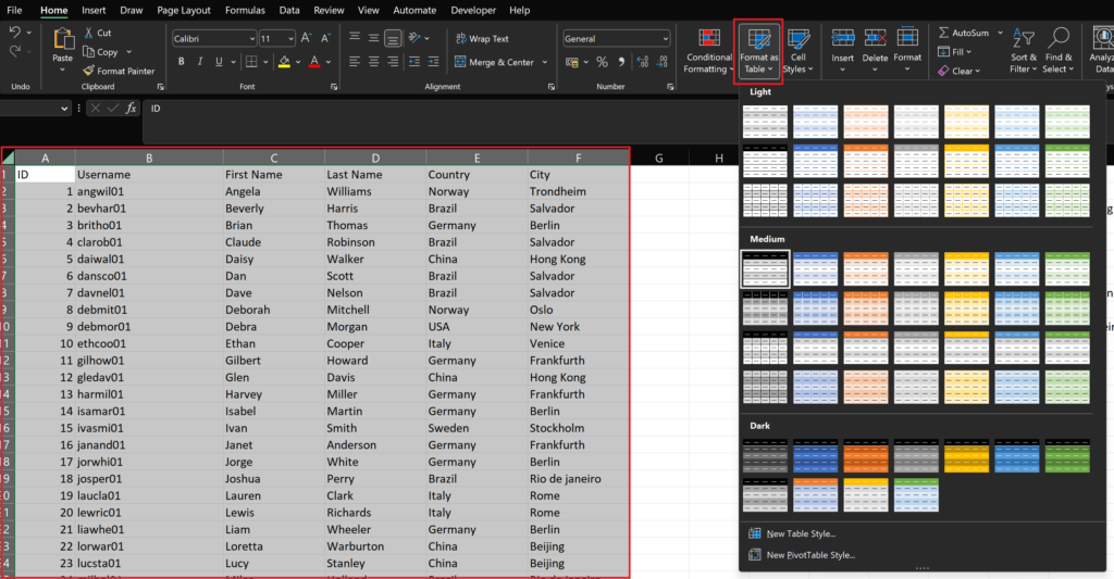
Now that we have a neat User table it’s time to make it a table. Select a color theme that you like!
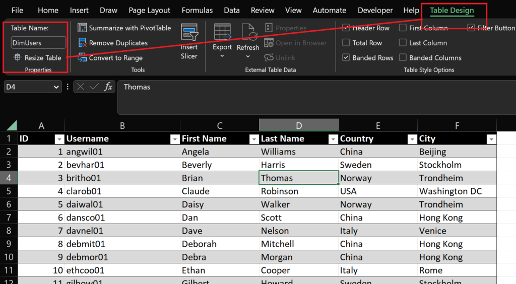
When selecting any cell in your table, you have the option to rename it here under Table Design.
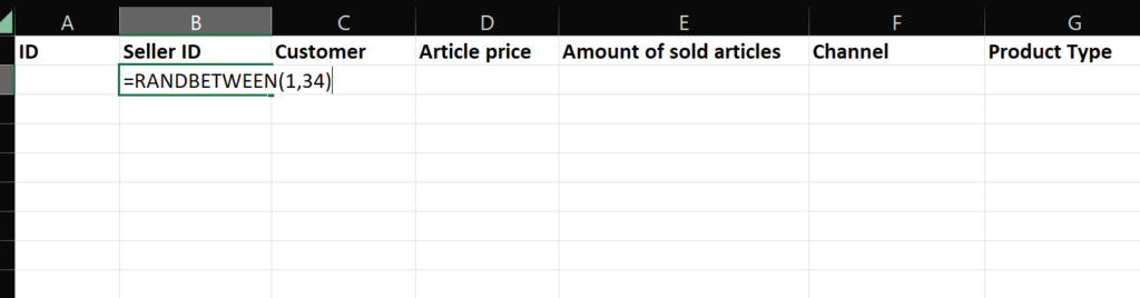
A Fact table
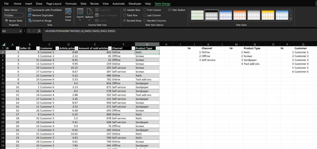
Next we’ll create a table of sales data that suits our needs. In my list of users I have 34 distinct records, so I’m just randomly select a number between 1 and 34.
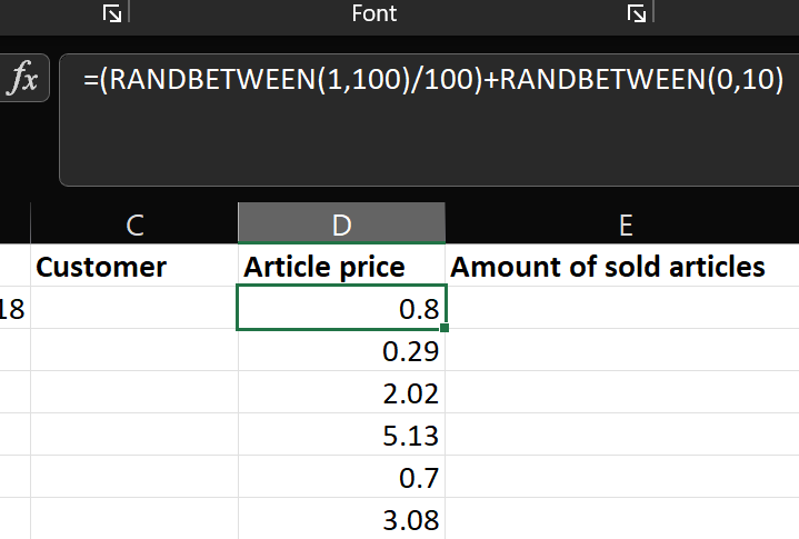
I want my article price to have decimals, so I make a random number between 1 and 100 and divide it by 100. There’s a 1% chance it becomes 100/100 meaning I will not have a decimal but that’s OK.
To increase the possible article price I now just add a whole number to our decimal number like this.
For Customer, you could make another dimension just like for the user or you can just add a name there using a simple XLOOKUP like we’ve done before here. Same procedure as before were we look up random values to add to our facts table.
When you’re done you can import it to Power BI and start visualizing!
Oh and let’s add a little tip. You can use an if statement with RANDBETWEEN to be a bit more selective with your facts table. If you for example want a certain product type to be represented more often you can use an if statement like this. Here I’m first randomizing a number between 1 and 100 and if it’s below 75 i.e. 75% of the times, I just write out Nails. otherwise I’m selecting one of the products by random, meaning that Nails might actually be selected again.
=IF(RANDBETWEEN(1,100)<75,"Nails",XLOOKUP(RANDBETWEEN(1,4),$M$2:$M$5,$N$2:$N$5))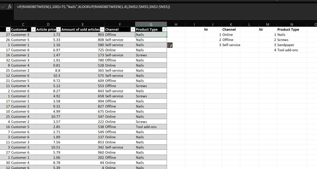
Now if you have read this far, you must be a real hard core Excel geek like me! Love it!
Just for you, I’m closing this off by adding even some more complexity to the previous formula where I kind of promised to not dive deeper 😉 What can I say? I lied.
What if you don’t only want 2 cities per country? What if Sweden has 3 possible cities and the other countries have 2. Now we need to randomize between the amount of cities that each country actually has.
Let’s switch out the 2 to to the amount of country rows found the the city table. A country with 14 possible cities will have 14 rows and thus we’ll randomly select from 1 to 14.
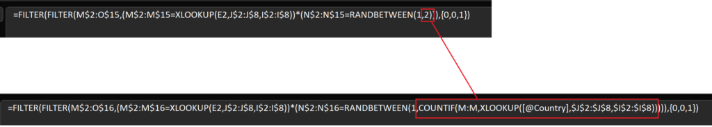
=FILTER(FILTER(M$2:O$16,(M$2:M$16=XLOOKUP(E2,J$2:J$8,I$2:I$8))*(N$2:N$16=RANDBETWEEN(1,COUNTIF(M:M,XLOOKUP([@Country],$J$2:$J$8,$I$2:$I$8))))),{0,0,1})Perhaps no more need to search for hours for that perfect dataset in order to showcase a Power BI report? Now you can like 20 minutes and impressing a lot of colleagues with your awesome Excel formulas while doing it 😉
Cheers!