Cross reference with Excel
Now and then, I get questioned about how to make cross references in Excel. Let’s say you have 2 lists and there are common values in both. You want to find for example usernames that exists in both lists. This post will explain how you achieve it using Xlookup. There is a more advanced way to do this using merge in Power Query, but I’ll save that for another blog post.
Let’s say we have this list available and want to cross reference them to determine who should get a pay raise based on the geekines for Excel.

How you do it
This method uses a formula in the table to look up the value from another table. Write out the formula in the cell as below. Select the value we’re looking for first.

Secondly we want to look in the C-column. We’ll bluntly just select all of these rows like this:

Whenever we find a matching row, we want whatever is on the same row from this column to be shown. In our case, whenever we find the name Tommy, we’ll grab what is says under “Is an Excel Geek” and put it it the cell we’re currently writing the formula in.

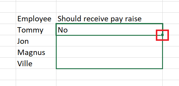
When done, hit Enter! To expand the formula downwards, drag from the corner and down like this:

This will copy the formula to the next cells. Excel is clever and will change the selected cell we’re searching for, for each row we copy the formula to. This means that for the next row, it will look in the same columns but search for “Jon” and then “Magnus” etc.

I was recommended this web site by my cousin. I’m not sure whether this post is written by him as nobody else know such detailed about my problem. You’re wonderful! Thanks!