Merging Cells in Excel lists
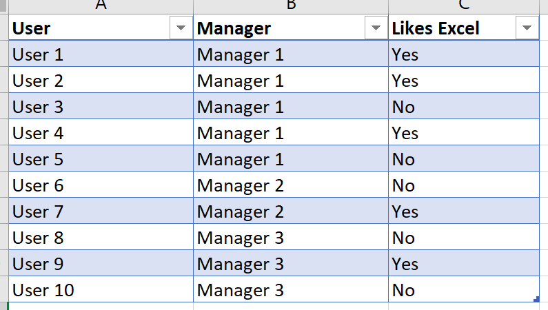
Lets say we have this list of people. We know who their managers are and we know whether they like Excel or not. (All users in this blog has given consent under GDPR to have their personal view on Excel processed).
Let’s say we want to send out an email (yes I know it’s old technology but bear with me on this one). We could just hook up our Excel file to a Word file and off we go! Super easy for us, not as valuable for the managers who will receive one email for every user in the list.
Instead let’s use good’ol Power Query! Select any cell in your table, go to Data and select “From table/Range”.

First of all, we’re only interested in the users that likes Excel, since we are going to suggest pay raises to the managers for some of their employed users. Let’s remove the other peasants.

With our new list of noble users, we no longer need this column so let’s remove it. We just want the user and manager column left for our next step.

Go ahead and click the “Group By” heading from the meny

Make sure you do the grouping by Manager, name your new field to whatever you want (we won’t keep it later either way) and make sure you don’t do any aggregations, but rather the Operation is set to “All rows”.

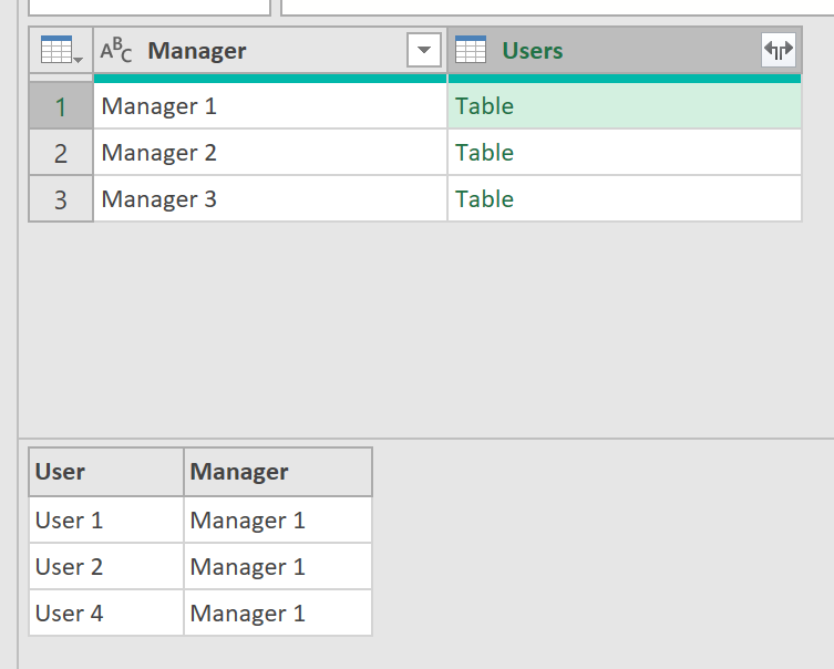
Since we choose all Rows, we get a table on each row with matching users! However we get the Manager once again in here and we already got enough managers, so lets just keep the users, shall we?
Create a new custom column and add this formula:
Table.RemoveColumns([Users],"Manager")

Hurray! Our Managers are gone! Your view should look something like this by now

Time to create yet another column! Oh, and as if things weren’t complicated enough already, I kind of lied before when naming our last column a “User List” when it was actually a Table, as you can see in the print screen above. Nothing good comes easy though and using this formula we can convert our table in to an actual list!
Table.ToList([User list])

Finally getting somewhere, right! Now your Power Query should look something like this.

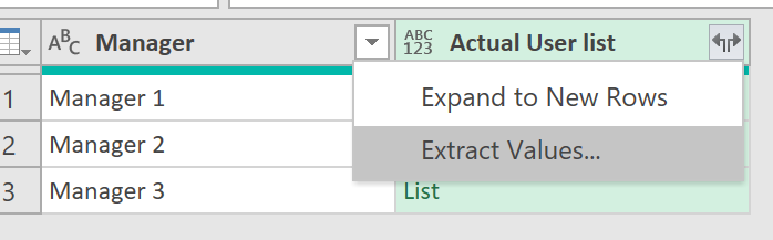
Remove the columns that have Tables in them and just keep the Manager and the Actual User list. Extract the values. If you have to much resources in your computer and want to waste some (as well as time), you can expand the user list to new Rows which will give you the exact same view as we began with! That way you get a chance to do all steps above once again. Or, you know, we could just extract the values and go on.
Here’s where the magic is about to happen! Select Custom delimiter in the list. This will expand the Extract values-window.

Using our new shiny options, select a Carriage Return from the list and it will populate the field with “#(cr)”. Hit that OK-button like your life depended on it!

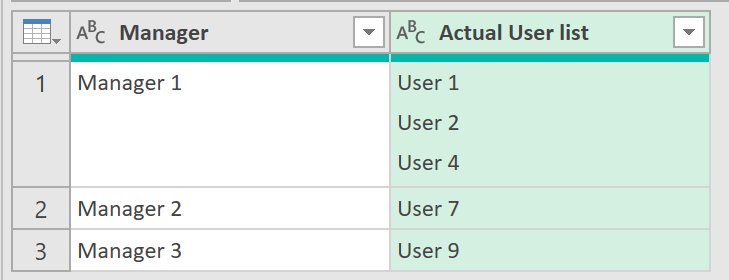
Voilá! A super neat list with all users in one cell and only 1 row per manager.
OK so now what? Well now you just hook up a Word file to this Excel table, write your information to the managers and tell them what users to increase paychecks for and hit the Send Email-button! The managers gets 1 email with a list of all their users instead of one email per user. Here’s how you do that last step!
Good luck! Stay productive out there!