Temperature Data in Power BI
I recently came into possession of a dataset of weather data from a friend of mine. Just as I am one of those normal friends who get’s thrilled when presented with 1,2 million rows of raw temperature data, so is he a very normal friend who gets thrilled by setting up home made temperature sensors and gather 1,2 million rows of data in a MySQL database. As we are going towards towards darker and colder times, me and Per can now take comfort in knowing how cold the upcoming times probably going to be. That is, if history is any kind of teller of the future. From the 22nd of August 2020 to the 29th of January 2021, a 160 days period, the temperature changed almost 63 degrees Celsius. It’s a good thing we humans are good at adapting!

I’m getting ahead of myself here. Let’s start at the beginning.
Transforming the data in Power Query
Per provided me with the external link to hes MySQL database server, the name of the database and finally an account with read access to the data. To get the data, you first need to install this connector for MySQL. Restart Power BI and we’re back in the game!
I first met this view of the date and timestamp as well as 1 column for each sensor and the temperature it had collected. One sensor had been added later so it had a bunch of blank rows and 2 sensors didn’t actually have any data.

Since I’ve previously made clear of my humanoid heritage, these column names where of little value. Fortunately you just need to double click on a headline to change it.
After renaming the sensors into human readable information, it look better! There’s just one issue. I like to say that if data looks simple to a human, it will be hard on Power BI. If it looks hard for a human, it will be simple for Power BI. This sounds like crazy talk, but you’ll see what I mean. We’ll take this:

And flip it using unpivot to look like this:
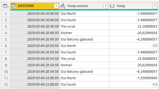
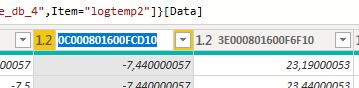
There is a neat and simple trick to get the names right in the Unpivot-step here. Make sure you have the Formula bar showing under the View-page and simply name the columns what you cant in the formula field after you’ve done the unpivot. By default it will otherwise be “Attribute” and “Value”.

We’re now done with transforming the data in Power Query! Let’s download it and make some further transformations in DAX!
Adding columns to the table
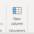
From our DateTime, I wanted a column that only show the date. We could have done this is Power Query but I prefer to only transform the data in there and add stuff in DAX so that the data load is a little bit faster. Creating a new column is done by clicking this button in the menu and then adding a formula for what the column should consist of.

My Date column looks like above. I also like to have a time only column. In Power BI, just like in Excel, dates are measured as whole days. We start on the 1900-01-01 and 1 1900-01-02. This means that 1 is actually 24 hours. 0,5 means 12 hours and so 0,5 as a date and time value would be 1900-01-01 12:00. What this means for us is that to get the time out of a date and time field, we want the decimal number.
We’ll get this by subtracting the whole date like this:
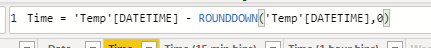
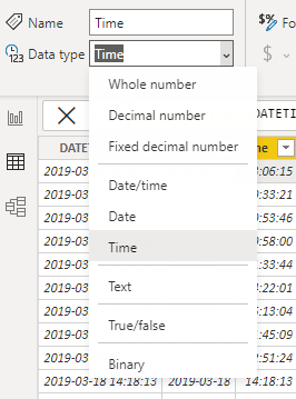
This rounds the date to 0 digits, meaning we strip away time and find ourselves with the value representing midnight of the date. We’ll end up with just the digits i.e. the time value. This will be a decimal number between 0 and 0,9 and we simply need to specify the column as a time column:
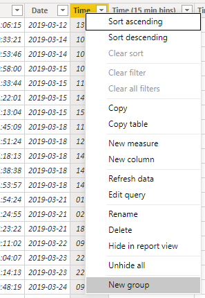
Now for some of that Power BI magic! We can group this information into bins like this:
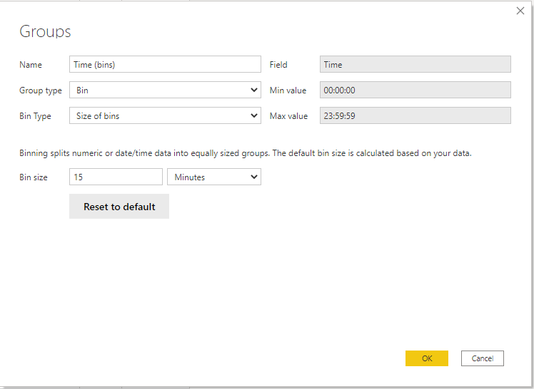
Now we can just specify the size of our Bin and click OK.
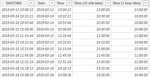
Behold! Our new columns are automatically calculated to a bin and if you want to visualize something by 15 minutes of by the hour, we’ll just use one of these columns.
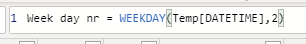
Next up – weekdays! By looking at the date, we can let Power BI tell us the week day number.
I’ve added the days manually in a column using the Switch function like this. In Power Query, you could also just add a column with the names of the days out of the box, but where’s the fun in that?

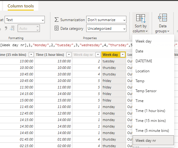
There is a reason I kept the week day nr as a column instead of putting it into the formula of the switch function. By selecting our new Week day-column and going to Column tools, I can tell Power BI to sort based on the number column. This will make sure Monday comes first instead of the days coming in alphabetic order.
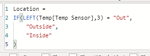
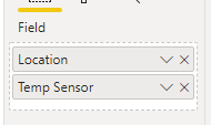
Our final column will be “Location” and it will tell us if the sensor is outside on inside by looking at the first 3 characters of the sensors name (which I happen to have named “Out” for the sensors that are outside).
Our new data set is complete!

Visualizing of the data
I began by creating this overview.

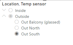
It felt like it made little sense comparing the outside temperature to the inside, so I’ve made a slicer with single select down to the left. The radio buttons only allow for one selection at the time. But hey! Friend of order might claim there are actually 4 selections made. This is possible due to stacking! By adding 2 fields on top of each other we can select in a form of main and sub menu.
Selecting one sensor will select that one only, but selecting the location “Outside” will automatically select all sub sensors as well. If this is not your desired outcome, simply make 2 slicers where you select inside or outside in one and the sensors in another.

By using the slicer we can change the entire layout of the overview like this and quickly get some neat insights! Sometimes you want to dig a bit though, which is why I created the “Over Time” page looking like this:

On the left we have the inside sensors, on the right we have the outside ones. On top we have the monthly avarage and in the bottom we see average over time of the day. Inside seems pretty stable but outside changes a lot! especially the glassed balcony that usually peaks around 15:00.
Now by selecting for example February in the Month slicer, we only show data from February but regardless of the year. We can see a decline in temperature between the year 2020 and 2021 on a monthly basis and the balcony was actually on average above 0 degrees for a few hours of the day.

Selecting 2021 as the year as well will tell us that the glassed balcony was probably a splendid refrigerator for most of the days in February that year.
When selecting a visualization on the page, you get the Format-tab and under there you can activate “Edit interaction”.
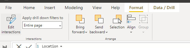
I’ve done this and then made it so that the indoor sensor graph does not have any power over the outdoor sensors and vice versa.

This is neat because I can click around in one of the graph and it won’t blank out the other one. If I had made this selection and interacted between the graphs (which by the way is one of the real super powers of Power BI), then the other graph would be blank since I’ve selected a sensor that does not exist in the left graph.

On this next page I’ve focused on days. The left graph show us the week days and the right graph show us the day of the month. During Q4 (regardless of year), the warmest outside temperature that occurred on a Thursday was 24,7 degrees.

One might also assume that Per was cooking some kind of celebration dinner at the end of the month of October. On the 30th the warmest temperature in the kitchen reached over 26 degrees from it’s average of about 22. The increase might be due to an oven opening. Who knows?

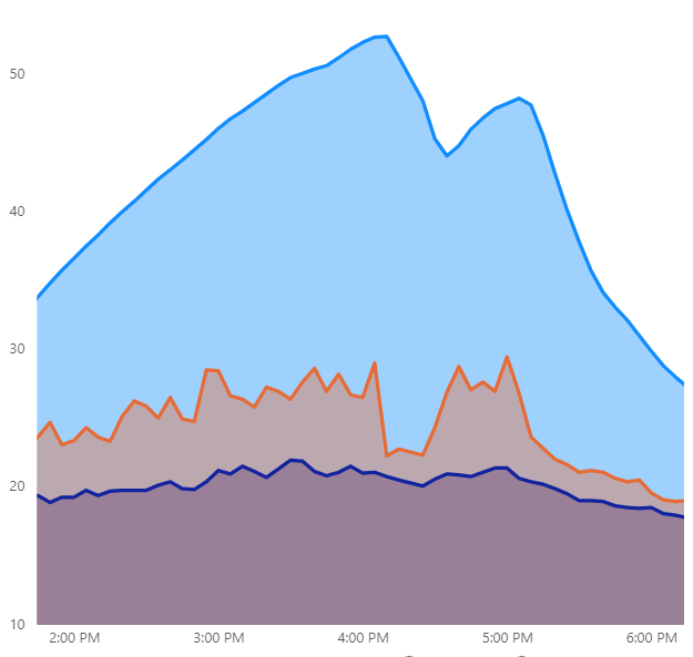
Next page is the Time of day. As before, the inside sensors are on the left and the outside are on the right.

On this graph you could actually change the X axis by yourself on the fly! These to arrows going down along side of each other will drill you to the next level.
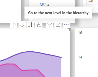
So what is the next level? Remember those bins we created earlier? I’ve stacked them in the Axis field like this. At first you will see a summarize by hour but you can drill down in granularity to 15 minutes or even 5 minutes with the touch of a button!
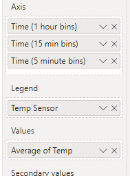
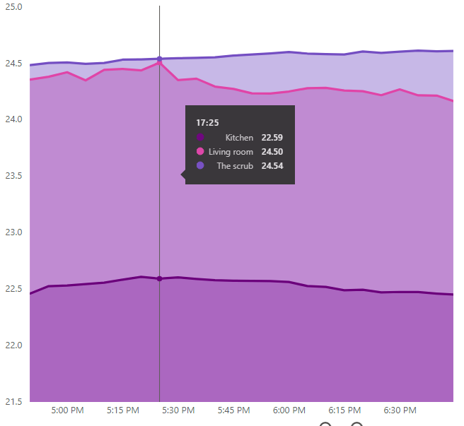
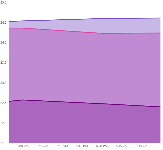
By pressing the arrows, the graph changes like this where we have 1 hour on the left, 15 minutes in the middle and 5 minutes on the right.

Why is this useful? Because we could have missed the slight increase of average temperature in the living room that seem to be happening at about 17:25 if we compare all the 64 measures that occurred at this time, because it cannot be seen in the hourly graph underneath! Knowledge would be lost! Chaos erupts! Thank god for grouping and stacking in Power BI!
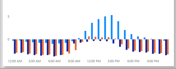
Finally we arrive at the extremes page! This is what we had a sneak peak of at the beginning of the blog post.

This view show us the extremes up and down. If we quickly want to know the warmest day of 2020, we can just select that year and boom – the 26 of February was the coldest day with almost -17 degrees Celsius of chills.

As the all knowing normal human friend I am (who totally didn’t click through the selections of sensors to find this out) I happen to know that it was coldest on the north sensor. By selecting that sensor as well, we can see that on this specific location in 2020, the warmest temperature was 32,5 degrees and it happened on the 27th of July. This meant a diff of almost 50 degrees!

Speaking of 50 degrees, that’s almost as warm is the warmest day in the glassed balcony! On the 9th of August in 2021

Going back to the time page and only selecting the 9th of August 2021, we can see that it didn’t stay this warm for more than about 45 minutes, but still pretty impressive heat there! The supreme refrigerator ability of the glassed balcony we saw in February would be less effective now to say the least.
And with that, the temperature report is completed! I’ve made a lot of insights here and I hope you learned something as well! And as always, if you have any questions feel free to reach out!
Cheers!