Scheduled refreshes from files
From time to time you might want to use an Excel or CSV file as the source for your Power BI reporting. The downside of doing so is that if you specify a local file as a source, the Power BI Service wont know how to access it after the report is published and so if there are changes in the files you cannot refresh the dataset.
There is however a simple workaround that I use quite often and in this short blog post I’d like to share how it’s done. There are more options to solve this of course and this is just one of them.
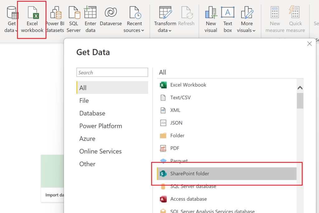
Allright first of, instead of using Excel as the source, select SharePoint Folder as your source. SharePoint Online is (as the name might suggest) an online source and thus the Power BI Service can refresh data from it.
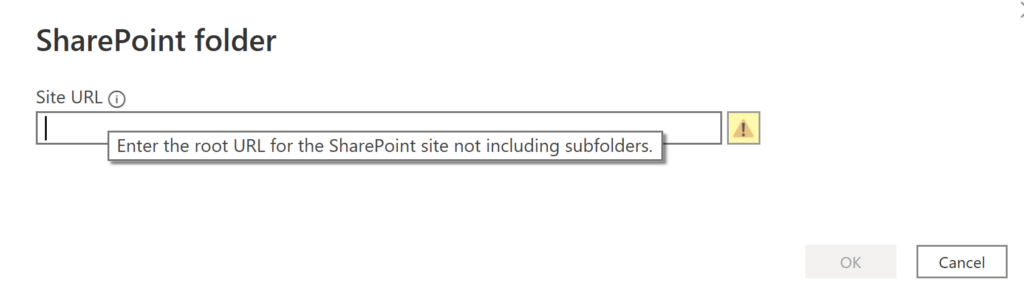
Next you enter the SharePoint site URL:
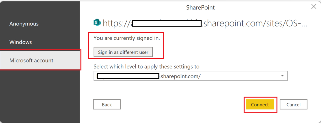
Use your Microsoft account to login.
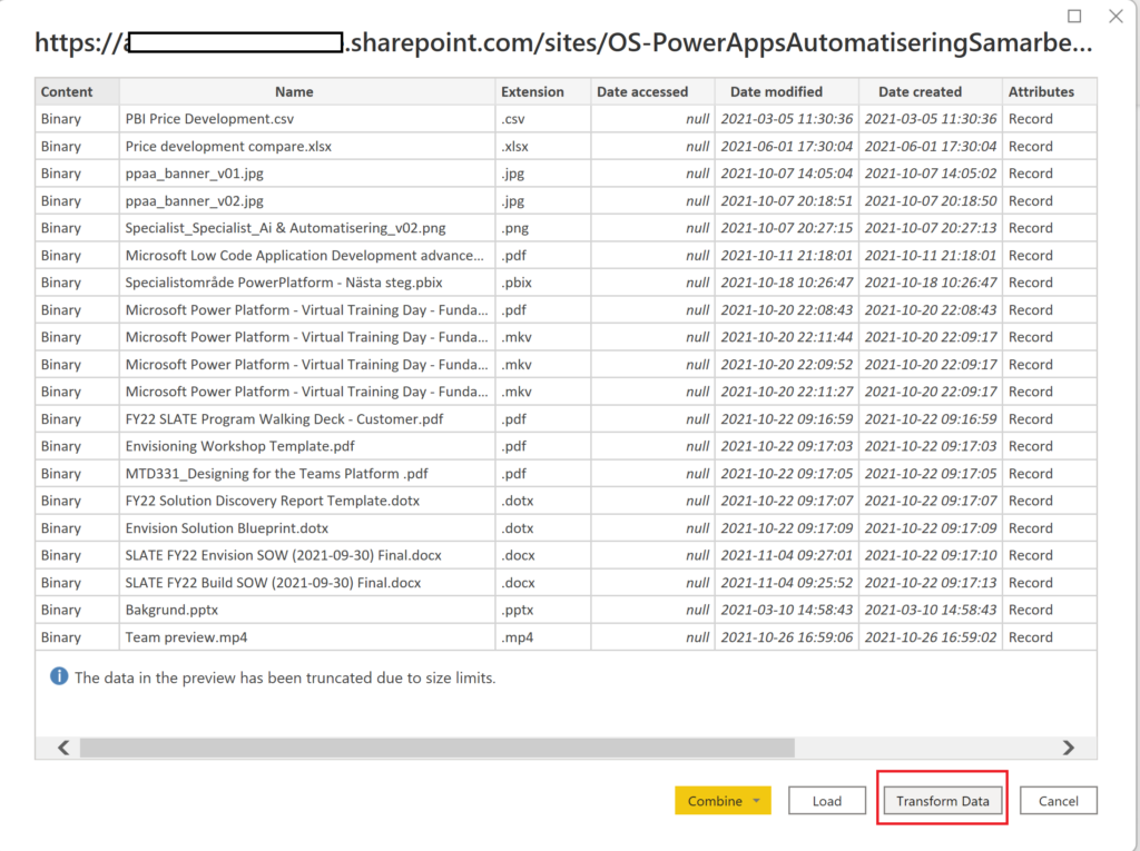
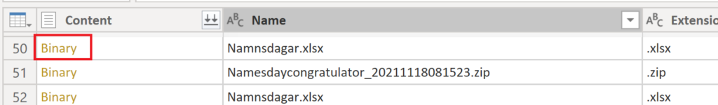
You will get a preview of all the files in the SharePoint site. Click Transform to open Power Query
Click on the binary for the file you want to open:
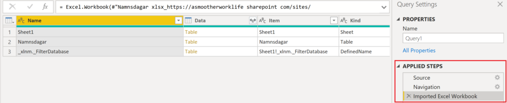
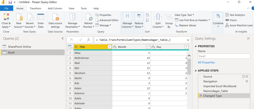
Voilá! You now have the sheets and tables of the Excelfile in front of you. 2 steps have been added to applied steps on the right as well. From here you can just select your data and get started doing your report building! After publishing the report to the Power BI Service you can schedule a refresh since the datasource is actually SharePoint Online, not the local Excel file. Do note that for this to work, the file must have the exact same name even if you change it’s content. You can change the file as well as long as the new file has the same name and structure.
What if I already connected to an Excelfile and have built a report?
Then you are doomed.
Nah just kidding! Let’s say you have a connection to your Excel file already in a query like this:
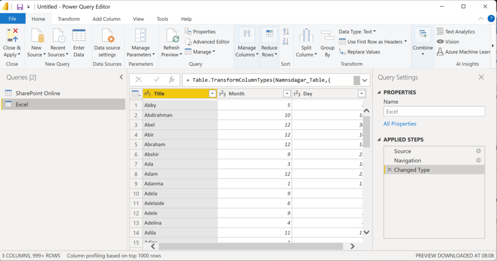
Note the applied steps on the right side. If you select the Source step, you’ll notice that it will show the available tables of the Excel file, just like the view that we ended up with from the SharePoint connection above.
Select the advanced editor to get the Power Query code (M). This way we can copy the applied steps from one query to another.
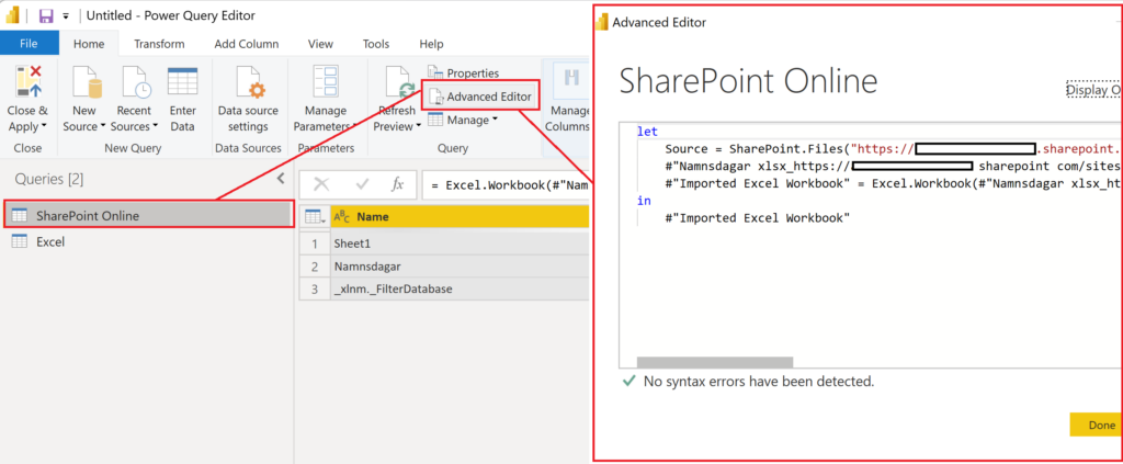
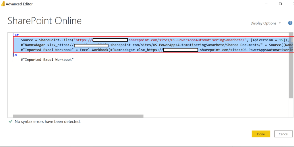
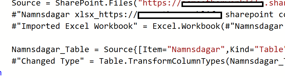
Next you will want to copy these three rows:
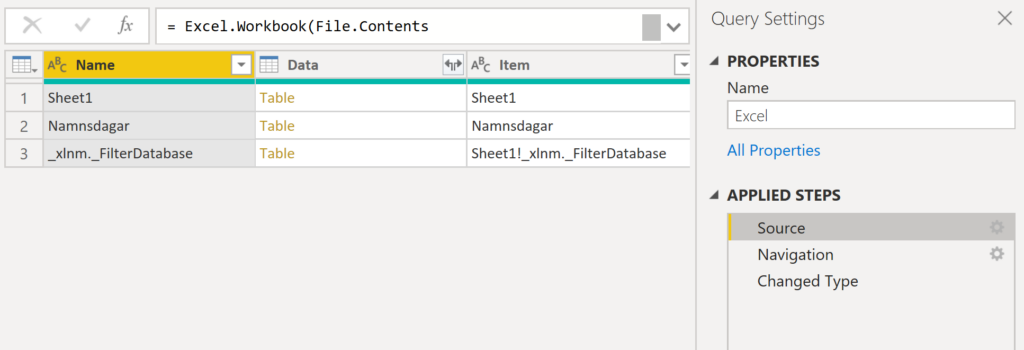
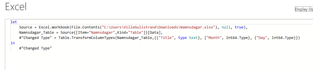
Head back to your query that goes directly to your Excelfile and open the advanced editor. It might look something like this.
Add your rows after the Source-row. You can comment the first row out so it’s kept but not used, using two front slashes.
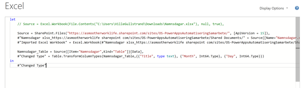
Remember to add a comma at the end of your pasted row. It was the last row of your previouse query but it’s not in this one.
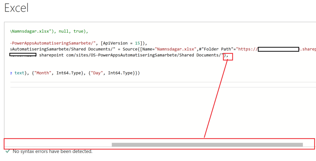
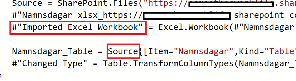
Next we need to make a final adjustment to the code. In Power Query, each row specifies the row before it and since we added new rows, we need to make this small change as well.
This is what the code looks like right now:
We want to change the Source-step to Imported Excel Workbook.
The new code looks like this:
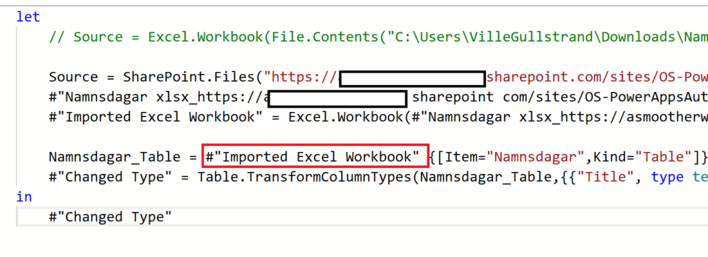
And that’s it! You’re done! You got a few more applied steps in the beginning of your query but you have successfully converted a local data source to an online data source!
If you have any questions feel free to reach out!
Cheers!